Differential Drive Robot Kinematics

TL;DR

Forward Velocity Kinematics

$\begin{bmatrix} \.x \\ \.y \\ \.\theta \end{bmatrix} = \begin{bmatrix}\frac{r}{2} && \frac{r}{2} \\ 0 && 0 \\ \frac{r}{L} && -\frac{r}{L} \end{bmatrix}\begin{bmatrix} \omega_l \\ \omega_r \end{bmatrix}$

Inverse Velocity Kinematics

$\begin{bmatrix} \omega_l \\ \omega_r \end{bmatrix} = \begin{bmatrix}\frac{1}r && 0 && \frac{L}{2r} \\ \frac{1}r && 0 && -\frac{L}{2r}\end{bmatrix} \begin{bmatrix}\.x \\ \.y \\ \.\theta \end{bmatrix}$

Introduction

A mobile robot operating in 3D space has 6 degrees of freedom expressed in terms of it’s pose: (x, y, z, roll, pitch, yaw). It is composed of two parts, the position (x, y, z) and the rotation (roll, pitch, yaw). Where roll, pitch and yaw are the rotations about the x, y and z axes, respectively.

For a planar mobile robot, the pose can be expressed as $(x, y, \theta)$ , where the position is given by $(x, y)$ and the heading is defined by $\theta$ . These three parameters are sufficient to describe the motion of a robot operating on a 2D surface.

A differential drive robot has wheels on either side of it’s body that can rotate independent of one another. The individual velocities of these wheels control the motion of the robot body on a planar surface. However, in order to accurately control the robot motion a mathematical model of the robot is required that calculates the resulting planar motion for given rotational wheel velocities, and vice versa.

The Kinematics Model

The kinematics model of a differential drive robot relates the rotational wheel velocities, $\omega_l$ and $\omega_r$ , to the planar robot motion, ( $\.x$ , $\.y$ , $\.\theta$ ). Where:

$\omega_l \text{: is the rotational velocity of the left wheel}$ $\omega_r \text{: is the rotational velocity of the right wheel}$ $\.x \text{: is the robot velocity in the x axis}$ $\.y \text{: is the robot velocity in the y axis}$ $\.\theta \text{: is the rotational velocity of the robot body}$

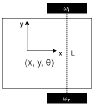
A typical differential drive robot is shown in the figure below. The robot pose is $(x, y, \theta)$ , the robot wheels have rotational velocities $\omega_l$ and $\omega_r$ and the distance between the wheels is $L$ .

The robot wheels have a radius of $r$ and they rotate with a rotational velocity $\omega$ .

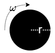
The resulting linear velocity from rotational velocity of the wheel is given by:

$v = \omega r$

It should be noted that when deriving the kinematics model we make the following assumptions:

The robot can only move in the direction of it’s x axis ( $\.x \ne 0 \text{, } \.y = 0$ ).
The wheels do not slide on the floor, all the movement is a result of the wheels rolling on the ground.

The robot motion is a combination of it’s translational movement ( $\.x$ ) and it’s rotational movement ( $\.\theta$ ). Therefore, we will study how the robot pose changes when we look into two extreme cases i.e., when the robot movement is purely translational and when the robot movement is purely roational.

Translational Movement

In this case both of the robot wheels spin with the same rotational speed and in the same direction, which causes the robot to move in the x axis.

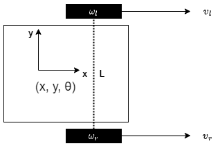
The rotaional velocity of each of the wheels can be converted into linear velocity as follows: $v_l = \omega_l r$ $v_r = \omega_r r$

Where $v_l$ and $v_r$ are the linear wheel velocities of the left and right wheel, respectively.

Since both wheels have the same linear velocity, it causes the robot to move in the x directions with no rotational speed. The velocity of the robot in the x axis is equal to the linear wheel velocities: $\.x = v_l = v_r$

Using this information we can derive the rotational velocities of the wheels as shown: $\omega_l = \frac {\.x}r$ $\omega_r = \frac {\.x}r$

Rotational Movement

In this case the rotational wheel velocities have the same magnitude but their direction is opposite. This causes the robot to rotate in one place i.e., the robot does not have any translational velocity but it has rotational velocity $\.\theta$ .

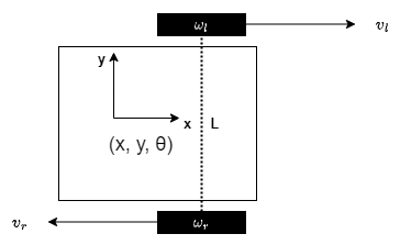
If we use the rotational velocity of the body to calculate the linear speed of the wheels, we get:

$\frac{L}2 \.\theta = v_l = \omega_l r$ $\frac{L}2 \.\theta = -v_r = -\omega_l r$

Which gives us:

$\omega_l = \frac{L}2 \frac{\.\theta}r$ $\omega_r = -\frac{L}2 \frac{\.\theta}r$

We have considered the purely rotational and purely translational cases, we can get all the possible velocities in between by controlling the rotation speed of the wheels and getting the linear combination of the two cases discussed above. After adding the equations we get:

$\omega_l = \frac {\.x}r + \frac{L}2 \frac{\.\theta}r$ $\omega_r = \frac {\.x}r - \frac{L}2 \frac{\.\theta}r$

The equations above defines the inverse velocity kinematics (IK) for the differential drive robot.

The forward velocity kinematics (FK) are as follows:

$\.x = \frac{r}2 (\omega_l + \omega_r)$ $\.\theta = \frac{r}L (\omega_l - \omega_r)$

In matrix notation, the IK can be written as: $\begin{bmatrix} \omega_l \\ \omega_r \end{bmatrix} = \begin{bmatrix}\frac{1}r && 0 && \frac{L}{2r} \\ \frac{1}r && 0 && -\frac{L}{2r}\end{bmatrix} \begin{bmatrix}\.x \\ \.y \\ \.\theta \end{bmatrix}$

and the FK:

Code

def FK():
    A = np.array([
              [r/2, r/2],
              [0, 0],
              [r/L, -r/L]
            ])

    B = np.array([
                [w_l],
                [w_r]
            ])

    return np.dot(A, B)

def IK():
    A = np.array([
              [1/r, 0, L/(2*r)],
              [1/r, 0, -L/(2*r)],
            ])

    B = np.array([
                [x_dot],
                [y_dot],
                [theta_dot]
            ])

    return np.dot(A, B)

TL;DR#

Introduction#

The Kinematics Model#

Translational Movement#

Rotational Movement#

Code#